Data management.

BIFLDA software is designed to process BIFL data obtained either from polarized measurements with the two detectors collecting 0 and 90 degrees traces (Polarization experiment) or from two detectors collecting two different colors (Two Color experiment). The software supports importing four detector data but the idea is to use every time just two of them. Things that can be analyzed are:
1) the polarizations of the two colors (same analysis as the polarized measurements),
2) the sum of two polarizations for each color (this is the magic angle trace: (s+2Gp)),
3) the total sum of all four detectors which is build up by summing the two magic angle traces from the two colors. The first analysis can be done separately for each color, the second and the third analysis is in fact the same as two-color experiment.

The source data that are imported by BIFLDA software are located either in one or in a series of files that have B&H SPC-402/432, SPC-401/431, SPC-6x0/256ch, SPC-6x0/4096ch, SPC-830 and other complementary to SPC-830 data formats (SPC-130/134, SPC-140/144, SPC-150/154) or in a file that have PicoQuant TimeHarp 200 (versions 5 and 6), PicoHarp 300 and Symphotime-64bit data format. Other data formats can be implemented upon request. One unit of data (BIFL data set) that can be imported at one step consists of up three sets of BIFL files:

1. first set of data files represents the continued sample BIFL trace;

2. second set of data files represents the continued scatter BIFL trace;

3. third set of data files represents the continued background BIFL trace.

It is also possible to use a part of sample BIFL trace as a background.

On the basis of imported BIFL data set for Two Color experiments the following three traces are built up:

• Channel 1 - trace containing the data from first detector.

• Channel 2 - trace containing data from the second detector.

• Total - trace containing data from the two detectors together. This trace is calculated from intensities of Channel 1 and Channel 2 as [channel1]+D*[channel2], where D is a correction for efficiency and wavelength dependence.

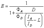
• Energy transfer efficiency (E) function according to the formula:

where:
D is the ratio between the different detector efficiencies. This parameter can be defined by user;
L is the proportion of the donor signal I_D leaking into the acceptor channel;
Ф_A and Ф_D the quantum yields of fluorescence for the acceptor and donor; I_D and I_A are the intensities of donor (channel 0) and acceptor (channel 1).

• Fractional intensity(F₂) function that is a measure for the emission maximum in a trace. This function is built according to the following formula:

where:
I₁ is intensity of channel 0;
I₂ is intensity of channel 1.

On the basis of imported BIFL data set for Polarization experiments the following five traces are built up:

• Channel 1 (S) - trace containing the data from first detector (S-polarized light).

• Channel 2 (P) - trace containing data from the second detector (P-polarized light).

• Total (Sum S + 2G*P) - trace containing data from the two detectors together. This trace is calculated from intensities of S and P as (S+2G*P).

• steady state polarization trace according the following formula

• steady state anisotropy trace according the following formula:

After building the required macrotime traces the BIFLDA software provides the possibility to create fluorescence decays and autocorrelation functions available for the fit and also inter arrival time distributions available for further IATD coincidence analysis. There is an option* to calculate absolute photon arrival times combining macro and micro time information**. Fluorescence decays and correlation functions are made only from Total-trace for the polarization measurements and from all traces for the two color measurements. Inter arrival time distributions can be calculated either from total trace or from each channel independently. There are three options for calculation of inter arrival time distributions from the total trace: independently from router, i.e. for each photon; for channel 1 to channel 2 time delay and for channel 2 to channel 1 time delay.
* absolute photon arrival times are always calculated for PicoQuant PicoHarp data.
**calculation of absolute photon arrival times can not be performed for PicoQuant TimeHarp data due to asynchronous macro time clock.

Building fluorescence decays, autocorrelations and IATD can be done from a selected time region (large time region) in the macro time trace. Visual selection of the time region with help of special data markers is possible. Sliding method for building fluorescence decays, autocorrelations and IATD from selected time region by either selected bursts or constant time shift or constant amount of photons is implemented.
It is possible to select large time regions in all macro time traces (Sample, Irf, Bg, and also Channel 1, Channel 2, Total) with help of data markers so that this time region is applied to all traces, but it is also possible to select manually different large time regions in each trace (sample, irf, bg). The sample irf and bg is operated freely. But within the sample (channel 1, channel 2 and total), the selected time region(s) is the same for all traces.

Building fluorescence decays.

Constant time shift or constant number of photons is possible to set for sliding. From the photons belonging to each small sliding time interval the separate decay is made.
To reduce number of channels and increase signal to noise ration fluorescence decays can be binned. Binning factor can be set by user (see Options/Binning).

Building autocorrelation functions.

Constant time shift or constant number of photons is possible to set for sliding. From the photons belonging to each small sliding time interval the autocorrelation function is calculated by either formula (*) or formula (**)

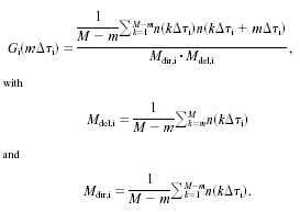
where j is the number of channel where correlation is calculated; M is total amount of channels; n is the number of photons in a bin, Dτ is a minimal time lag. The bin width (time lag) can be set by user.
An alternative formula ** is used when quasi-logarithmic time scale is set.

Building anisotropy decays.

For each small sliding time region a time resolved anisotropy decay is built by the formula

The only time resolved anisotropy decays are displayed (in the case of polarization measurements in solution). Decays of S and P are not plotted.

Building inter arrival time distributions.

Solution experiment data management scheme.

In this case experiment was done in solution and not immobilized on coverglass or polymer. The measurement is the actual Burst Integrated Fluorescence. A molecule passes the focus and generates a burst. These burst can be detected by software. Therefore minimum and maximum thresholds is set. Minimum to discriminate between dark noise and a burst, maximum threshold to discriminate between single molecule passing through focus or two or more at same time giving rise to higher intensity. Intention is to select in this way only those burst coming from single molecule.

The selection of bursts can be done in total trace and applied also to S and P. The same procedure is valid for two color experiment (first selection in the total trace and then applied to color 1 and color 2).

Sliding analysis in this case will occur over several bursts. All photons from different burst can be used if put one after each other (no combinations of photons from different bursts are used for building autocorrelation).

Analysis algorithms

BIFLDA software provides the possibility to fit single fluorescence decays, anisotropy decays and autocorrelation functions described in previous section. Global analysis is not supported. One fit session can process fluorescence decays or correlation functions or anisotropy decays built from one macro-trace. In case of two color experiment, in one fit session three decays or autocorrelation functions built from channel0, channel1 and total macro-traces are fitted. It is possible to uncheck any of characteristics mentioned above in order to prevent them from being analyzed.

Analysis of all fluorescence decays, autocorrelation functions and anisotropy decays is done using MLE method with multinomial statistics.

The MLE method with multinomial statistics consists of target fit criterion and optimization method. Target fit criterion is defined by the following formula:

where:
x_i - measured curve;
y(a) - theoretical curve calculated with corresponding model;
v - number of degrees of freedom;
 

The Marquard-Levenberg algorithm is used as the standard minimization algorithm for MLE.

Analysis of fluorescence decays:

Analysis of fluorescence decays is done using theoretical model of following general form:

where parameters δ, b, γ and c can be fitted by the software.

The multiexponential model is used as a pure fit model. This model is defined by the following equation:

where:
N is number of exponents;
p_j and τ_j are amplitudes and fluorescence lifetimes that can be fitted.

Analysis of anisotropy decays:

Analysis of anisotropy decays is done using the following theoretical model:

where  r₀, φ and are parameters to be fitted;

The software fits the anisotropy decays calculated from BIFL data (see data management section) directly using the formula mentioned above.

Analysis of autocorrelation functions:

Analysis of autocorrelation functions is done using the following theoretical model:

where:
c_k and τ_k are amplitudes and triplet lifetimes that should be fitted;
M is number of exponents in the sum.

In the case if autocorrelation function was built with FCS experiment the following model is used for fitting:

where are parameters to be fitted;

In the case if fluorescence decays, anisotropy decays and autocorrelation functions were prepared from BIFL data without applying sliding method they are analyzed independently one by one.

In the case if sliding method was used the following analysis steps are performed during one fit session:

1. initial curve prepared from a separate macro-time region (see Data management section) is analyzed with a corresponding model. In the case of fluorescence decays analysis on this step parameters δ, b, γ and c are fitted. Also the start and end channels for analysis are defined on this step;

2. curves prepared from sliding window are analyzed automatically one after another. The start and end channels for analysis are taken from previous step and are same for all curves analyzed on this step. In the case of fluorescence decays analysis on this step parameters δ, b are fixed to the values obtained on the previous step. For each fluorescence decay analyzed on this stage parameters γ and c are fixed to different values. These values are obtained by multiplying values of parameters γ and c taken from step 1 by ratio of time duration of sliding window to time duration of large time region. Also before starting analysis on this step the values of all parameters obtained on step 1 can be changed by user manually.

Generation of initial guesses for model parameters can be enabled and disabled. Manually entered fit parameter values (in a case of disabled initial guesses) as well as minimum and maximum constrains keeps the same while analyzing all curves during one fit session. In the case if sliding analysis method is applied generation of initial guesses is performed automatically for both initial decay and sliding decays prepared from sliding window.

The measured fluorescence decays can be fitted to theoretical models with and without convolution.

After fit is done the weighted residuals and their autocorrelation function are calculated.

IATD coincidence analysis (by Weston et al. 2002)

Bursts selection

Bursts can be selected automatically or manually either in intensity or in time lag macro time plot. At first step one has to apply Lee smoothing filter. Lee filtration is described as following. The raw data n_k with n_k being the number of photons (count numbers) in the bin k of the macrotime trace with 1<=k<=N can be smoothed by a Lee filter of window width 2m+1 which is defined as follows: first a running mean and variance are calculated using

 , m<k<=N-m
 , 2m<k<=N-2m
The range of the k values is limited by the window width. The filtered data  are given by